A commodity credit book can change in minutes, not days. If I want tighter control, I need three things working together: live prices for intraday MtM and limit checks, historical data for PD/LGD and stress testing, and a clean audit trail so every number can be traced back to its source.
Here’s the short version:
- Live spot prices update exposure and collateral values during the day.
- Webhook alerts flag warning and breach events soon after market moves.
- Historical OHLC data supports volatility, Z-scores, VaR, PD, and LGD work.
- Forward curves and correlations help estimate future exposure and basis risk.
- Validation rules block stale, mismatched, or spoofed data before it hits models.
- Governance cycles keep intraday controls, model reviews, and approval steps on the right schedule.
A few numbers make the point clear: price feeds can update every 1 to 5 minutes, webhook notices can arrive in about 10 seconds, and long-run historical series can go back to 1990. That mix lets me track today’s exposure while still testing what happens under shocks like 2008, 2020, or 2022.
| Input | Main job in credit risk |
|---|---|
| Live prices | Intraday MtM, exposure, collateral checks |
| Historical prices | Volatility, VaR, PD/LGD calibration |
| Analytics | Stress signals, regime checks, correlation review |
| Forward curves | Future exposure estimates on open positions |
| Alerts and logs | Limit monitoring, audit trail, review workflow |
In plain terms, this article shows how API data moves through one loop: ingest data, validate it, value positions, monitor limits, run stress tests, and update models.
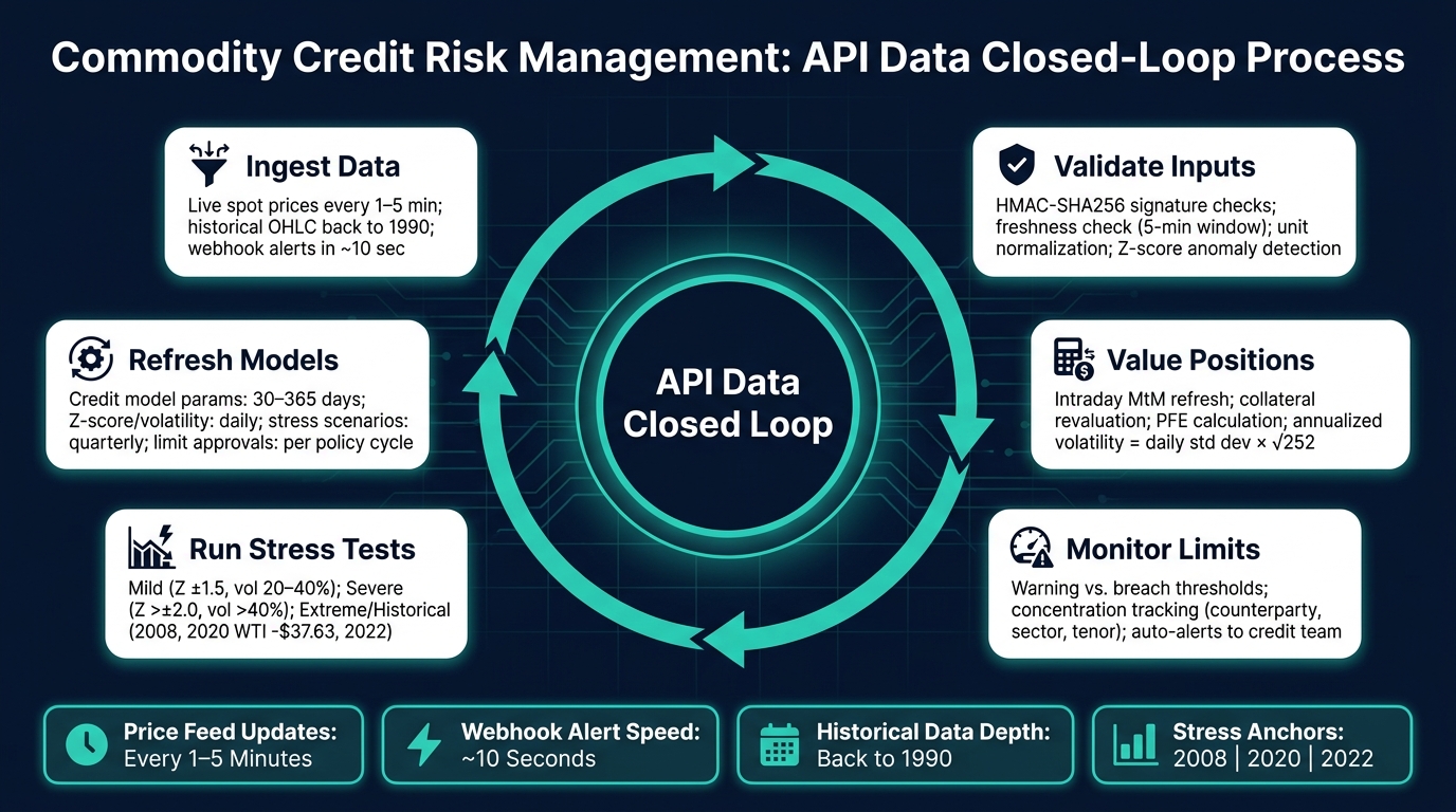
Commodity Credit Risk Management: API Data Closed-Loop Process
Data Inputs for Credit Monitoring and Exposure Calculation
Exposure starts with clean, mapped data.
Map Live Prices to Contracts, Inventories, and Customer Positions
Each price feed needs to connect to a contract, inventory line, or customer position. In day-to-day work, that usually means using standard commodity codes like BRENT_CRUDE_USD, WTI_USD, NATURAL_GAS_USD, and GOLD_USD to tie API responses back to internal contract IDs and customer positions. That link sets the flow: price feed → contract mapping → position valuation → exposure.
Unit consistency matters across the whole book. Crude oil may come in as USD/barrel (bbl), natural gas as USD/MMBtu, gold as USD/troy ounce (oz), and diesel as USD/gallon (gal). The API’s unit field gives you a clean way to check those conversions before bad math slips into valuation.
For E&P names, rig counts and production data can add extra credit signals on top of market prices.
Once those feeds are linked to positions, exposure can be recalculated at the contract level.
Use Historical Series for Trend, Volatility, and Regime Analysis
Daily OHLC history back to 1990 for major benchmarks gives credit teams enough data to measure rolling volatility and build stress-period benchmarks. A 20-day or 50-day SMA can help flag regime shifts and possible collateral pressure, while annualized volatility helps size limits. The formula is simple: annualized volatility = daily return standard deviation × √252.
Z-scores below -2 or above 2 can flag stress and feed into PD adjustments. In plain English, these signals help shape collateral thresholds, PD model inputs, and limit headroom decisions.
Of course, none of that helps if the source data is wrong at the start.
Build a Clean Ingestion and Validation Layer
The validation layer should run before exposure calculations. Think of it as a credit-control gate: if the data is stale, mismatched, or spoofed, it shouldn’t reach the model.
| Check Category | What to Validate |
|---|---|
| Normalization | Map commodity codes to internal contract IDs and confirm units match contract terms |
| Integrity | Verify HMAC-SHA256 signatures on webhook payloads to prevent spoofing |
| Freshness | Reject stale data if updated_at falls outside the 5-minute refresh window |
| Analytics | Use rolling volatility and Z-scores to spot anomalies before model ingestion |
Store timestamps in ISO 8601 UTC, such as 2026-07-12T13:10:43Z, to support audit trails. For failed webhook deliveries, use exponential backoff.
With clean inputs in place, the next step is intraday MtM and limit monitoring.
sbb-itb-a92d0a3
Live Exposure Updates and Limit Monitoring
Once clean, checked data is in place, the next job is keeping exposure numbers up to date during the trading day, not just at end-of-day settlement.
Refresh MtM and Collateral Coverage Intraday
Prices move intraday, so MtM valuations need to move with them. With the /v1/prices/latest endpoint, credit teams can map each new price to open contracts, hedges, and inventory positions, then refresh MtM valuations, potential future exposure (PFE), and unsecured balances in near real time.
The same logic applies to collateral. Live price feeds also revalue borrowing-base assets like stored inventory, which means collateral coverage can shift fast when markets move. That can turn a comfortable position into a tight one in a hurry.
A few controls help keep that process tight:
- Webhook alerts can send limit events to the credit team in near real time.
- Volatility bands can be used to tighten intraday margin rules.
- OilpriceAPI's analytics API can surface volatility metrics directly, which makes this easier to automate.
Track Concentration, Limit Utilization, and Breach Alerts
Teams should also watch counterparty, sector, and tenor concentration at the portfolio level. After each MtM refresh, compare the updated exposure with policy limits.
Alerts should fire automatically when exposure crosses policy thresholds. It helps to split those into warning and breach levels so teams get a heads-up before pressure turns into a limit event. Webhooks can manage both levels.
| Metric | Warning Level | Breach / Alert Level | Credit Team Action |
|---|---|---|---|
| Annualized Volatility | 20%–40% | > 40% | Increase MtM frequency; tighten margin terms |
When a breach happens, it should go into the same credit workflow already used for exposure review. Each alert should include contract IDs and desk codes. Critical breaches should also be sent to the ETRM audit trail and an instant message channel so credit, trading, and operations are all looking at the same signal at the same time.
Historical Data for Default, Loss, and Stress Testing
After intraday exposure control, historical data helps turn live market signals into default and loss estimates. Historical price series support PD, LGD, expected loss, and stress testing.
Calibrate PD, LGD, and Expected Loss Using Historical Price Data
Use daily OHLC returns to calibrate stress scenarios and loss models.
Tie historical downturns to each counterparty's actual cash flow structure. That matters because a price drop on a chart doesn't tell you much by itself. The key is what that move does to debt service, collateral value, and liquidity. For example, Brent crude fell from $115 to $46 per barrel in six months during the 2014 U.S. shale boom. Run that full path through the counterparty's cash flow model to measure how cash flow coverage erodes and when breaches begin.
Z-scores add context for stressed collateral values and borrower cash flows. High/Low ranges help capture intraday gaps that closing prices can miss in LGD calibration.
Those calibrated loss inputs then feed straight into the stress cases below.
Run Scenario Analysis for Price Shocks and Prolonged Downturns
Map each scenario to a price regime and its portfolio effect.
| Scenario Level | Z-Score Range | Annualized Volatility | Portfolio Impact |
|---|---|---|---|
| Mild Stress | ±1.5 | 20%–40% | Prices at the 25th/75th percentile; potential for minor limit utilization increases |
| Severe Stress | > 2.0 or < -2.0 | > 40% | Significant over/undervaluation; high risk of collateral shortfalls and counterparty defaults |
| Extreme / Historical | N/A | Extreme | Market dislocation, such as WTI at -$37.63 in April 2020; likely widespread limit breaches and liquidity pressure |
Anchor each scenario to a named historical event - 2008, 2020, or 2022 - so assumptions stay auditable.
The next step is to test what happens when market shocks and counterparty weakness land together.
Test Portfolio Resilience Under Combined Market and Counterparty Stress
Real losses often come from linked market and credit effects. A market shock can hit exposure at the same time it cuts into a counterparty's ability to repay.
Combined stress tests should also account for basis risk. The Brent-WTI spread can widen sharply during geopolitical stress, creating losses in portfolios hedged to one benchmark but exposed to another. Correlation analysis helps track whether that link still holds under joint stress scenarios.
Let the counterparty's own cash flow sensitivity move with the shock. If revenue is tied to crude prices, the stressed PD should rise as the price scenario gets worse instead of staying fixed at the base case. Pull historical series through the API and simulate the joint path of price, exposure, and credit deterioration.
Use these outputs as inputs to model refresh and validation controls.
Model Refresh, Governance, and the Credit Control Loop
Set Refresh Cycles for Data, Models, and Approvals
After stress testing, the main job changes. It’s no longer about building scenarios. It’s about deciding how often each control should update.
Not every control should run on the same clock. MtM needs intraday spot prices. Threshold breaches need fast alerts. Supply-side inputs and model inputs can update more slowly. To cut down on false alerts, use cooldown periods such as 60 minutes and only send notifications when predefined threshold moves occur. Supply-side indicators like rig counts update weekly, and drilled-uncompleted (DUC) well inventories update monthly, so they fit longer-term credit modeling better than intraday exposure tracking.
| Model or Approval Input | Refresh Interval | Governance Purpose |
|---|---|---|
| Credit Model Parameters | 30–365 days (rolling) | Keep models aligned with current market regimes |
| Z-Score / Volatility Metrics | Daily or on threshold breach | Trigger out-of-cycle credit reviews |
| Stress Scenario Assumptions | Quarterly or after major events | Maintain calibration to named historical events |
| Limit Approvals | Per policy cycle or breach event | Ensure limits reflect current exposure and risk appetite |
Credit models should refresh on a defined cycle. Metrics such as Z-scores, percentiles, and annualized volatility should be recalculated over 30- to 365-day windows so models stay aligned with current market regimes. A Z-score beyond ±2.0 can trigger an out-of-cycle credit review.
Fast refresh sounds good on paper. But it only helps if every update is traceable and repeatable.
Maintain Validation, Audit Trails, and Change Management
Once refresh timing is in place, the next step is simple: prove that every input can be audited and reproduced.
Every credit input needs a traceable source and timestamp. The governance goal is versioned inputs, reproducible calculations, and audit-ready logs that risk committees and internal audit can use to reconstruct past decisions.
Keep historical versions and data logs available so past calculations can be reproduced on demand. Standardized error handling and exponential backoff retries help maintain system reliability during transient outages. API usage should also be monitored to avoid data gaps that could blind the credit monitoring system.
Conclusion: Build a Closed-Loop Credit Process with API Data
Live API price feeds make exposure calculations more accurate and timely. Historical series and analytics give credit model calibration and stress tests a factual base. Disciplined refresh cycles - intraday for exposure, defined periods for model review, and event-driven for ad hoc checks - keep decisions current without adding extra noise. Cryptographic data validation and versioned audit trails make each calculation defensible for regulatory reporting and internal review. API data creates a closed loop: ingestion updates exposure, exposure resets limits, limits trigger stress tests, and stress tests refresh models.
FAQs
How do live API prices improve intraday credit control?
Live API data makes intraday credit control much sharper because it delivers the real-time prices needed to keep portfolio valuation and exposure checks up to date throughout the trading day.
With live feeds from OilpriceAPI, risk systems can automatically refresh position values, recalculate VaR and other exposure metrics, and flag credit-limit breaches as soon as market conditions shift. That means teams can react faster instead of waiting for the next batch update. In volatile periods, that speed can help cut intraday loss risk.
What checks should run before prices reach risk models?
Before prices make their way into risk models, do some basic quality and integrity checks. That step helps you avoid shaky outputs and bad calls later.
Check that the data is fresh by looking at metadata. Confirm the request came back clean by reviewing response status fields. And make sure the dataset lines up with your plan limits, permissions, and product needs.
It also helps to verify source semantics, especially for futures data, where contract details and field meaning can trip you up fast. Review the time series to make sure it’s complete, with no missing points or odd gaps. Then confirm the JSON structure matches what your application expects before sending anything into downstream VaR, sensitivity, or Monte Carlo analysis.
How does historical commodity data support PD and LGD estimates?
Historical commodity data helps support PD and LGD estimates because it gives analysts the raw input they need for volatility modeling, stress tests, and scenario analysis.
With OilpriceAPI’s historical price data, teams can run Monte Carlo simulations, calculate VaR, and study how prices moved in the past. That makes it easier to estimate default probability, gauge potential losses, size hedges, and set risk limits with more precision.