Crude seasonality can help you read the market, but it will not tell you where price goes next. If I were using this guide today, on July 9, 2026, I’d treat it as a simple workflow: pull long-run Brent and WTI price data from an API, clean and align the dates, group prices by time of year, and then check whether the Brent-WTI spread is moving in line with past seasonal patterns or far away from them.
Here’s the short version:
- I’d use daily data for spread checks and short-term moves.
- I’d use monthly averages to study recurring seasonal shape with less day-to-day noise.
- I’d convert API timestamps from UTC to America/New_York before merging the two benchmarks.
- I’d check for missing dates, duplicates, outliers, and roll-related jumps before doing any analysis.
- I’d compare summer driving season, refinery maintenance periods, and winter heating season instead of looking at the full year as one block.
- I’d treat a spread or price move with a Z-score above +2 or below -2 as a sign to inspect it, not as an automatic trading signal.
- I’d keep in mind that OPEC+ moves, wars, sanctions, and supply shocks can overwhelm normal seasonal demand patterns fast.
A few facts stand out. The guide notes that Brent often trades at a $2.00 to $5.00 premium to WTI, and that Brent history can go back to 1976, while WTI can go back to 1983 through the API discussed. It also points out that about 20% of global oil trade moves through the Strait of Hormuz, which helps explain why supply risk can outweigh seasonal demand at any time.
If you want the plain takeaway, it’s this: use seasonality for context. Look at what usually happens in May through August, September through October, November through February, and March through April. Then compare that baseline with current inventories, refinery runs, and supply headlines before you make any call.
Demand, Supply and the Seasonality of Crude Oil
Quick comparison
| Topic | WTI | Brent |
|---|---|---|
| Main market link | U.S. inland demand | Global seaborne demand |
| Seasonal sensitivity | Often shows summer gasoline demand more clearly | Often reflects global heating and supply pressure more |
| Exchange link | NYMEX | ICE |
| Spread reference | Usually the lower leg in Brent minus WTI | Often trades at a premium of about $2.00 to $5.00 |
| Best use in this workflow | U.S. demand and refinery-run seasonality | Global demand and seaborne pricing checks |
So before I trust any seasonal pattern, I’d first ask one simple question: is this a normal demand-period move, or is supply driving the market instead?
Set Up Brent and WTI Seasonal Data With an API
Pull Historical Brent and WTI Prices From OilpriceAPI
Start with clean, aligned Brent and WTI price history. OilpriceAPI offers a JSON REST API with Brent data back to 1976 and WTI data back to 1983, which gives you a long enough runway to test seasonal patterns across very different market regimes.
To pull a historical series, use the GET /v1/prices/historical endpoint with these four parameters:
| Parameter | Value | Notes |
|---|---|---|
by_code |
WTI_USD or BRENT_CRUDE_USD |
One request per benchmark |
interval |
daily or monthly |
Daily for spreads; monthly for trend models |
start_date |
e.g., 1983-01-01 |
YYYY-MM-DD format |
end_date |
e.g., 2026-07-09 |
YYYY-MM-DD format |
Each JSON response includes the fields you need for seasonal analysis: price (raw float), formatted (display string like "$74.52"), currency, code, and created_at (ISO 8601 timestamp). Use price for calculations. Save formatted only for display.
"Daily data supports volatility and spread analysis." - OilpriceAPI
Use daily intervals when you want to compare spreads or measure short-window volatility. Use monthly intervals for ARIMA models or long-range trend decomposition.
Normalize Timestamps, Units, and Storage
The API returns timestamps in UTC, such as 2025-12-29T15:30:00.000Z. Convert those timestamps to America/New_York, then normalize each record to the trading date before you merge the series. Since all prices are quoted in USD per barrel, check that the currency field is USD before you store anything.
WTI trades on NYMEX, while Brent trades on ICE, so their holiday calendars don’t line up perfectly. That small mismatch can throw off spread work if you ignore it. For Brent-WTI spread analysis, build a shared date index, load both series into a pandas DataFrame, join on date, and deal with holiday gaps before calculating spreads.
Store the raw price field after converting UTC timestamps to America/New_York and verifying USD. CSV, Parquet, and PostgreSQL all work fine for this step.
Run Basic Data Quality Checks Before Analysis
Before you group by season or calculate spreads, run four checks on every data pull.
Missing dates can skew seasonality. Check for gaps on shared trading days and make sure the full date range is present.
Duplicate rows can skew averages too. They often show up after reruns, so look for repeated (date, code) pairs and remove them before analysis.
Outliers can throw off spread work, but they need review, not blind deletion. Use Z-scores to flag values beyond ±2 standard deviations, then inspect those records before deciding what to do with them.
Contract rolls can create fake jumps in futures data and distort trend signals. Watch for sharp moves around delivery-month transitions and review those periods before you include them in seasonal calculations.
With both series aligned, move to decomposition.
sbb-itb-a92d0a3
Apply Time-Series Methods to Measure Seasonality
Decompose Trend, Seasonality, and Noise
Once the series line up, split each one into three parts: a long-term trend, a seasonal component, and irregular shocks like outages or demand shocks.
The additive vs. multiplicative choice is pretty simple when you look at how the seasonal move behaves.
- Use additive decomposition when the seasonal move stays about the same in dollar terms no matter where crude is trading.
- Use multiplicative decomposition when the seasonal move grows or shrinks with the price level. So a 5% summer demand bump hits a lot harder at $100/bbl than at $40/bbl.
For crude, STL (Seasonal-Trend decomposition using LOESS) is often the better pick. Simple moving-average decomposition can be too rigid. STL does a better job with outliers and shifting seasonality. Run STL on both Brent and WTI, then compare the seasonal piece from each series.
| Method | Best Use Case | How It Handles Shocks |
|---|---|---|
| Additive | Constant seasonal swings in dollar terms | Shocks absorbed into the residual |
| Multiplicative | Seasonal swings proportional to price level | Shocks scaled by trend and season |
| STL | Volatile markets with outliers | Robustly isolates shocks from trend |
Use the same decomposition method for Brent and WTI so the seasonal components can be compared directly.
Use Rolling Windows and Structural Break Checks
Next, check if Brent and WTI seasonality still holds up when the market changes. Big regime shifts can bend or blur seasonal signals.
A practical way to handle this is rolling-window analysis. Instead of fitting one model across the full history, calculate seasonal averages in overlapping windows and compare them over time. If a recurring peak keeps showing up window after window, it’s more likely to be a durable pattern. If that peak fades in a later window, you may be looking at a regime shift instead of a stable seasonal effect.
It also helps to pair that with a structural break check. Split the sample into pre-break and post-break periods, then compare the seasonal shape across both parts.
Use those period-by-period results before you group the series by season.
Implement the Workflow in Python or R
Run the same process for both benchmarks so the output stays apples-to-apples. In Python, a compact workflow with pandas and statsmodels covers most of the job.
After pulling data from OilpriceAPI and loading it into a DataFrame with a datetime index, resample daily closes into monthly averages with df["price"].resample("M").mean(). Monthly averages cut down day-to-day noise and make seasonality easier to compare.
Then group by calendar month. df.groupby(df.index.month).mean() gives the average price or return for each month across the full sample. After that, use statsmodels.tsa.seasonal.STL to pull out the trend, seasonal, and residual components.
If you work in R, stl() and the feasts package in the tidyverts ecosystem give you the same type of workflow with similar syntax.
Use Z-scores only to flag months that drift away from the seasonal pattern. And before you do any spread analysis, make sure both benchmarks use the same cleaned index.
Group by Season, Analyze Brent-WTI Spreads, and Plan Charts
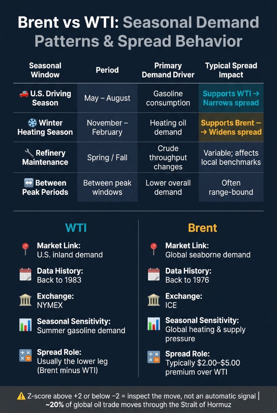
Brent vs WTI: Seasonal Demand Patterns & Spread Behavior
Build Seasonal Groups for Prices and Returns
Once you've identified the seasonal component, use it to sort the trend output into comparable time windows. The goal is simple: line up the parts of the year that tend to move for the same demand reasons. Use the same seasonal windows defined earlier so the analysis stays consistent from one step to the next.
For each seasonal group, calculate:
- average price
- median return
- standard deviation
- interquartile range (IQR)
The mean and median show the center of the data. The standard deviation and IQR show how far values move around that center. A tighter IQR points to a more repeatable seasonal pattern. A wider IQR usually means more noise, or a higher chance of shock-driven moves.
Carry these same seasonal windows into the spread analysis too. That way, you're comparing like with like instead of mixing demand regimes.
Measure Seasonal Behavior in the Brent-WTI Spread
The Brent-WTI spread is Brent minus WTI, expressed in USD per barrel. Track how that spread widens or narrows across each season.
Season matters here. During the U.S. driving season, stronger gasoline demand can support WTI and narrow the spread. In Q4, heating demand and tighter seaborne supply can favor Brent and widen the spread. Refinery maintenance in spring and fall can also move the spread, but that effect tends to be less consistent.
| Seasonal Window | Period | Primary Demand Driver | Typical Spread Impact |
|---|---|---|---|
| U.S. Driving Season | May – August | Gasoline consumption | Supports WTI and narrows the spread |
| Winter Heating Season | November – February | Heating oil demand | Supports Brent and widens the spread |
| Refinery Maintenance | Spring / Fall | Crude throughput changes | Variable; affects local benchmarks |
| Between peak-demand periods | Between peak windows | Lower overall demand | Often range-bound |
To spot unusual spread behavior, use Z-scores. Readings above +2.0 or below −2.0 usually point to a shock rather than a seasonal move. You can pull spread metrics such as mean, min, max, and Z-score from OilpriceAPI’s /v1/analytics/spread?spread=wti_brent endpoint.
Use Clear Chart Structures and Summary Tables
Use the same seasonal labels in both charts and tables. That sounds small, but it makes the whole analysis easier to scan.
Seasonal line charts help you compare the same window across different years, which is useful for checking whether peaks and dips show up again and again. Monthly box plots help from another angle: they show the full distribution of prices or returns for each month, not just the average.
Pair each chart with a summary table that includes season, average Brent and WTI prices, and spread stats:
- mean
- median
- min
- max
That gives finance and engineering teams a fast reference point without forcing them to dig through every chart.
Read Seasonal Signals Carefully and Wrap Up
Know the Main Limits of Crude Seasonality
Seasonal patterns in crude oil do matter. But they don't operate in a vacuum.
Crude prices are pushed around by several forces, and any one of them can drown out a seasonal pattern fast. In practice, no single factor stays in control for long. OPEC+ production decisions, including quota changes and voluntary cuts, are seen as the biggest driver of oil price forecasts, and they often override seasonality.
Geopolitical shocks can do the same thing. Brent crude jumped to $139 per barrel in March 2022 after Russia invaded Ukraine. That move came from supply fears and sanctions, not from the time of year. The Strait of Hormuz moves about 20% of global oil trade, so even threats around that route can spark sharp volatility.
Long-term market shifts matter too. U.S. shale output and changes in Chinese demand, including EV adoption, can reshape old seasonal patterns over time. That's why Brent-WTI and crack spreads should be used here as a final check, not as the main story.
Use Seasonality as Context, Not a Forecast
Seasonal analysis works best when it sits next to current fundamentals, not in place of them.
A simple way to think about it: seasonality gives you a baseline, not a call on where price goes next. It shows what has tended to happen during a certain part of the year. It does not tell you what must happen now.
To make that baseline useful, layer in current data such as:
- inventories
- refinery runs
- rig counts
- OPEC+ decisions
Use Z-scores to spot moves that sit far from seasonal norms. And when volatility is high, seasonal signals tend to get weaker, so any read based on them deserves more doubt. After a major regime shift, re-test the seasonal pattern instead of assuming the old one still holds. Also, avoid fitting short, odd samples too tightly.
With those limits in place, the workflow becomes a reading tool, not a forecast engine.
Conclusion: A Practical Workflow for Seasonal Crude Analysis
In day-to-day use, this workflow helps you sort evidence. It does not tell you direction with certainty.
Clean data from OilpriceAPI, seasonal decomposition, and spread checks can give you context. That's the point. The key habit all the way through is to treat seasonal patterns as informative, not predictive.
FAQs
How much history is enough for crude seasonality?
For seasonal demand analysis, at least 3 years of daily data is usually enough to spot and chart recurring patterns.
That said, OilpriceAPI goes much further back. You can access Brent data back to 1976 and WTI data back to 1983.
Why does that matter? Because a longer price history gives you a better view across very different market regimes, including price runs, crashes, and range-bound periods.
Should I analyze spot prices or returns?
Returns are often a better way to assess volatility, run backtests, and analyze trends in crude oil markets. When you convert spot prices into returns, you normalize the data and cut down price-level bias.
That matters because it makes benchmark comparisons, like WTI vs. Brent, much cleaner. It also helps with more accurate seasonal demand modeling. You can pull historical spot prices from OilpriceAPI and then convert them into periodic returns.
When should I trust spread seasonality less?
Put less weight on spread seasonality when big non-seasonal forces are throwing old patterns off course, such as:
- geopolitical events
- OPEC+ quota changes or voluntary cuts
- big shifts in U.S. shale output
- unexpected demand swings
Seasonal trends are just one input. Oil prices move in a global market, and they’re tied to things like U.S. dollar strength too. That’s why it helps to compare any seasonal signal with the current forward curve.