If scale control is weak, a gas well can lose flow, lose rate, and lose money fast. In U.S. gas production, that risk matters a lot because shale gas makes up about 75% of total output, or roughly 90–95 Bcf/d.
Here’s the short version: good scale inhibitor injection starts with the right well data, not the chemical truck. If I were explaining this guide in plain terms, I’d say it shows you how to:
- spot when a gas well has scale risk
- choose between continuous injection, batch treatment, and squeeze treatment
- design a squeeze job around water load, temperature, gas rate, and chemistry history
- track post-job results using gas production, water production, inhibitor dose, and producing days
- check whether a treatment failed because of low dose or a well/mechanical issue
- tie results back to $ / MMBtu gas price and treatment ROI
- set up clean data flows for well IDs, timestamps, lab data, and market prices
The main point is simple: if you match treatment design to water production and reservoir conditions, then monitor the right post-job signals, you can make better calls on retreatment timing and well ranking.
Scale Inhibitor Squeeze Application
sbb-itb-a92d0a3
Quick comparison
| Method | Best use | Main tradeoff |
|---|---|---|
| Continuous injection | Wells with stable water flow and surface access | Needs regular chemical feed at surface |
| Batch treatment | Wells that can be treated from time to time | Shorter life between jobs |
| Squeeze treatment | Wells that need longer life between treatments | More design work and shut-in time |
What you’ll get from this guide:
- a plain-English view of how scale forms in gas-well systems
- the field steps behind preflush, placement, overflush, and soak time
- the warning signs that show a squeeze may be fading
- a simple way to think about cost vs. preserved gas production
- data setup tips so treatment results can be tracked well over time
In short, this guide moves from scale chemistry to field execution to production and revenue tracking without getting lost in filler.
Scale Formation and Injection Methods
How Scale Forms in Gas-Well Systems
Scale forms when produced-water chemistry becomes unstable. As fluids move up the wellbore, pressure drops and temperature changes can push dissolved minerals past their solubility limits.
In gas wells, most inorganic scale comes from three main triggers: pressure drop, temperature change, and brine mixing. This shows up a lot in hydraulically fractured wells, where injected fluids come into contact with native brine.
Once you know the scale risk, the next step is picking the right way to get inhibitor into the well.
Continuous, Batch, and Squeeze Injection Compared
Operators usually have three main ways to deliver scale inhibitor into a gas well. The right method depends on well access, completion design, water rate, and how long the treatment needs to last.
| Method | Best fit |
|---|---|
| Continuous injection | Wells with steady water rates and reliable surface access |
| Batch treatment | Wells suited to periodic intervention |
| Squeeze treatment | Wells needing longer inhibitor life between treatments |
If treatment life is the main priority, squeeze design usually becomes the go-to option.
Squeeze Design and Field Execution
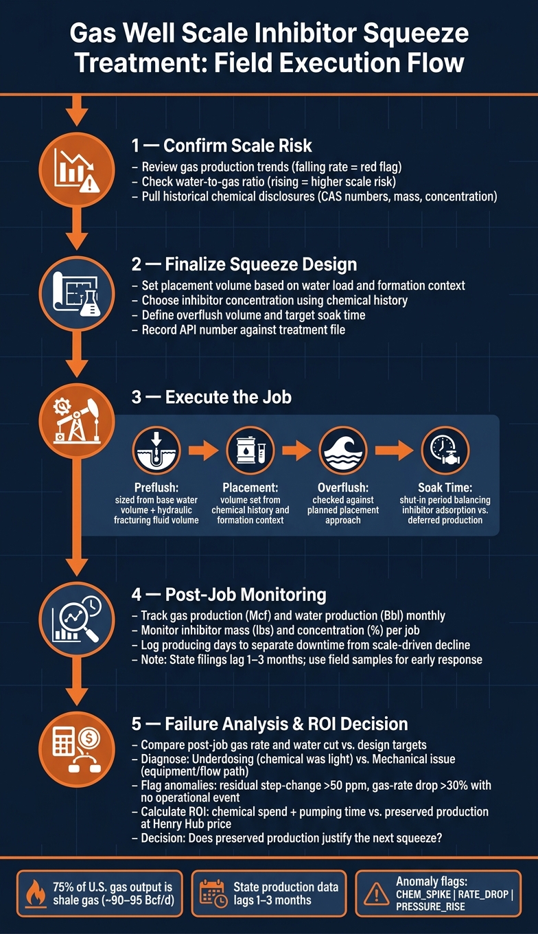
Gas Well Scale Inhibitor Squeeze Treatment: Step-by-Step Field Execution Guide
Once squeeze treatment is the chosen method, the design details decide how long the job holds up.
Key Inputs for Squeeze Design
Squeeze design starts with well data, not the pump truck. Those inputs shape placement volume, inhibitor loading, and retreatment interval. Put simply, the main drivers are water load, temperature, and prior chemistry.
| Data Category | Specific Inputs | Impact on Design |
|---|---|---|
| Produced Water | Water volume, producing days | Determines squeeze life and retreatment frequency |
| Gas Production | Gas rate, water-to-gas ratio | Influences inhibitor concentration and placement strategy |
| Chemical History | CAS number, chemical mass, concentration | Guides inhibitor selection and compatibility checks |
| Reservoir Context | Formation, typical depth | Informs temperature-stability requirements |
| Well Identity | API number, operator name | Used to track treatment history and candidate selection |
Bottomhole temperature matters because reservoir temperature and pressure affect inhibitor stability. Water rate is the main driver of squeeze life, since inhibitor depletion tracks with water throughput.
Historical chemical disclosures also help narrow the inhibitor choice. CAS numbers, mass, and concentration can all serve as anchors during design work.
Those inputs flow straight into decisions around preflush, placement, overflush, and soak time.
Preflush, Placement, Overflush, and Soak Time
A squeeze job moves through four stages, and each one has a clear purpose.
Preflush comes first. Size it using total base water volume and hydraulic fracturing fluid volume.
Placement comes next. Placement volume is set from available chemical history and formation context.
Overflush is sized as part of the total fluid plan and checked against the planned placement approach before the job starts.
Soak time is the shut-in period before the well goes back on production. It should balance inhibitor adsorption against deferred production.
Candidate Selection and Execution Steps
Not every well needs a squeeze. The biggest payoff usually comes from picking the right wells first.
Start with production trend analysis. Wells with falling gas rates and steady or climbing water volumes are the clearest signal for review. A high water-to-gas ratio is another strong flag.
Field execution usually follows this sequence:
- Confirm scale risk - review production trends and historical chemical disclosures to confirm that treatment is needed.
- Finalize the design - set placement volume, inhibitor concentration, overflush volume, and target soak time.
- Record the API number against the treatment file.
- Execute the job - check actual pumped mass and total fluid volumes against design specs during pumping.
- Begin post-job monitoring - sample produced water and track gas and water trends after restart.
State production data can lag by one to three months, so field samples are the better way to check early treatment response.
After restart, the focus moves from pumping the job to tracking how the well responds.
Monitoring, Failure Analysis, and Economics
Monitoring Data That Matter
After a squeeze job restarts, production data tells you one simple thing: is the treatment still working or not?
Two signals usually stand out first: gas production (Mcf) and water production (Bbl). If gas rates keep slipping while water volume moves up, that can be a sign that scale is restricting flow.
Here are the main signals to watch and what each one helps you decide:
| Signal | Source | Update Frequency | Decision Supported |
|---|---|---|---|
| Gas Production (Mcf) | State filings | Monthly | Identify flow restrictions and scaling trends |
| Water Production (Bbl) | State filings | Monthly | Monitor water-to-gas ratios and scaling risk |
| Inhibitor Mass (lbs) | FracFocus Registry | Per Job / Monthly | Verify dosing accuracy and program compliance |
| Inhibitor Concentration (%) | FracFocus Registry | Per Job / Monthly | Identify underdosing or incompatibility |
| Producing Days | Operator Reports / State filings | Monthly | Separate production declines from downtime |
| Natural gas price ($/MMBtu) | Henry Hub / Market Feeds | Real-time / Daily | Measure treatment value and program economics |
State filings lag one to three months; use internal monitoring for immediate decisions.
The pre-job baseline matters just as much after the treatment as it did before it. Without that benchmark, it's hard to tell whether a dip in gas rate is normal decline, downtime, or a squeeze that is starting to wear off.
Common Failure Patterns and How to Diagnose Them
Most squeeze failures show up first in production behavior, not in a lab report. A falling gas rate and a change in water cut are often the first clues.
To sort out what went wrong, compare post-job results with the treatment plan. Focus on:
- Post-job gas rate
- Water cut
- Pumped inhibitor mass
- Downtime
That side-by-side check helps separate underdosing from mechanical trouble. If the chemical program was light, the squeeze may fade early. If dosing looked right but production still drops, the issue may be tied to equipment, flow path damage, or another operating problem.
Water-to-gas ratio is especially useful after restart. Since scale comes from produced water, a rising water cut can point to higher scaling risk and may signal the need for more inhibitor or shorter treatment intervals.
Once the failure mode is pinned down, the next step is straightforward: compare treatment cost with the production it helped keep online.
Treatment Costs and Value Tracking
This part comes down to dollars and volume. What did the treatment cost, and how much gas did it save?
On the cost side, include chemical spend plus pumping time or intervention time. On the value side, count preserved production and avoided workovers. That's the trade-off.
To estimate ROI, operators start with a production baseline built from historical monthly filings. Then they measure how much gas rate was preserved after the treatment. At the current Henry Hub price, even a modest amount of preserved production can stack up fast.
Tracking producing_days each month also helps teams avoid bad calls. If production falls because the well was offline for a workover, that's not the same as a scale-driven decline. Operator reports and state filings help make that distinction clear.
In plain terms, the monthly review is trying to answer one question: did the squeeze preserve enough production to make the next one worth doing?
Data Pipelines and Conclusion
How to Structure Scale-Treatment Data Pipelines
If you want treatment results to lead to repeatable analysis, the data has to be set up the right way from the start. Put the fields needed to compare design, execution, residuals, and post-job performance under a single well ID and timestamp. That means pulling together well metadata, treatment events, lab results, and the production metrics used in post-treatment analysis.
Bring job logs, lab exports, and SCADA or historian feeds into one schema. Standardize timestamps to ISO 8601 and UTC, but keep local time-zone metadata for reporting. Convert volumes to bbl, pressures to psig, temperatures to °F, and residuals to ppm. Treatment labels also need to stay consistent: Scale Squeeze, Continuous Injection, and Batch Treatment. That way, downstream analysis can compare wells without messy naming issues. And one more thing: treat null as missing data, not zero.
Bad data should not slip into the main workflow. Flag out-of-range residuals, negative rates, and samples that fall outside a well's on-stream window, then send them to a quarantine table. To line up samples, treatment events, and SCADA data, use a shared time index at the minute or hour level with nearest-neighbor or time-window matching.
A simple warehouse layout usually works best:
- Raw object storage
- Curated warehouse tables for well master
- Treatment events
- Lab results
- Production and operations
Add anomaly flags on top of that structure. They help spot early signs of squeeze fade, underdosing, or pressure problems. For example, a residual step-change greater than 50 ppm, a gas-rate drop greater than 30% with no recorded operational event, or an unexpected pressure increase can trigger flags such as CHEM_SPIKE, RATE_DROP, and PRESSURE_RISE.
Using Market Price Data in Analytics Workflows
Once the technical pipeline is in place, market prices can sit on top of it as a separate context layer. Use OilpriceAPI's JSON REST API for real-time and historical natural gas prices, then store that data in a dedicated Market Prices table keyed by date/time and commodity.
From there, join gas prices to production windows to estimate incremental revenue tied to longer squeeze life. That makes it easier to rank wells by expected dollar value instead of looking at treatment data in isolation.
Conclusion
After the data is standardized, the same pipeline can support day-to-day operations and economic analysis. A clean setup turns treatment, residual, and production data into faster, better scale-control decisions.
FAQs
How do I know if a gas well is a good squeeze candidate?
Review the well’s production history and fluid chemistry for signs of mineral deposition. Use OilpriceAPI well-production endpoints to assess performance and track water-production trends, which can line up with scale formation.
You can also check FracFocus disclosure records through OilpriceAPI to see whether specific chemical additives, such as scale inhibitors, were used during completion. Put those two data sources side by side, and you get a clearer read on the problem: whether production drops are more likely tied to scale buildup or to reservoir depletion.
What causes a scale squeeze treatment to fail early?
The sources provided do not cover the technical reasons behind early scale squeeze treatment failure in gas wells.
Instead, they deal with OilPriceAPI data and services, including:
- FracFocus chemical disclosure data
- U.S. well production records
- Natural gas storage reports
So, based on these sources alone, there isn't enough information to explain why a scale squeeze treatment might fail early in a gas well.
How should I measure the ROI of scale inhibitor injection?
Compare treatment costs against production gains or avoided losses at the well level. Use monthly oil, gas, and water volumes to spot declines tied to scale and to verify recovery after treatment.
Look at the total cost of ownership, including:
- Chemical
- Equipment
- Labor
Then compare that spend with added revenue from sustained flow rates. Pull commodity data from OilPriceAPI so the analysis uses current natural gas pricing.