If I want a commodity model to do more than react to noise, I need features, not just raw prices. For short forecasts, I’d lean on lags, EMA, momentum, ROC, volatility, and z-scores. For medium windows, I’d add rolling means, seasonality, spreads, and detrended residuals.
Here’s the short version:
- Raw prices drift. Returns and normalized inputs are often easier for models to use.
- Short horizons like 1 to 5 trading days usually fit shorter windows such as 5, 7, 10, or 14 days.
- Medium horizons like 2 to 8 weeks often fit 20-, 30-, 50-, or 90-day windows.
- In commodities, I also need to watch for trading-day alignment, holiday gaps, and front-month roll effects.
- A few features do a lot of the heavy lifting: trend, momentum, volatility, seasonality, and spreads.
The 10 features covered are:
- Lagged prices and returns
- Rolling mean
- Exponential moving average (EMA)
- Momentum
- Rate of change (ROC)
- Rolling volatility
- Rolling z-score
- Seasonality flags
- Spread changes
- Trend and detrended residuals
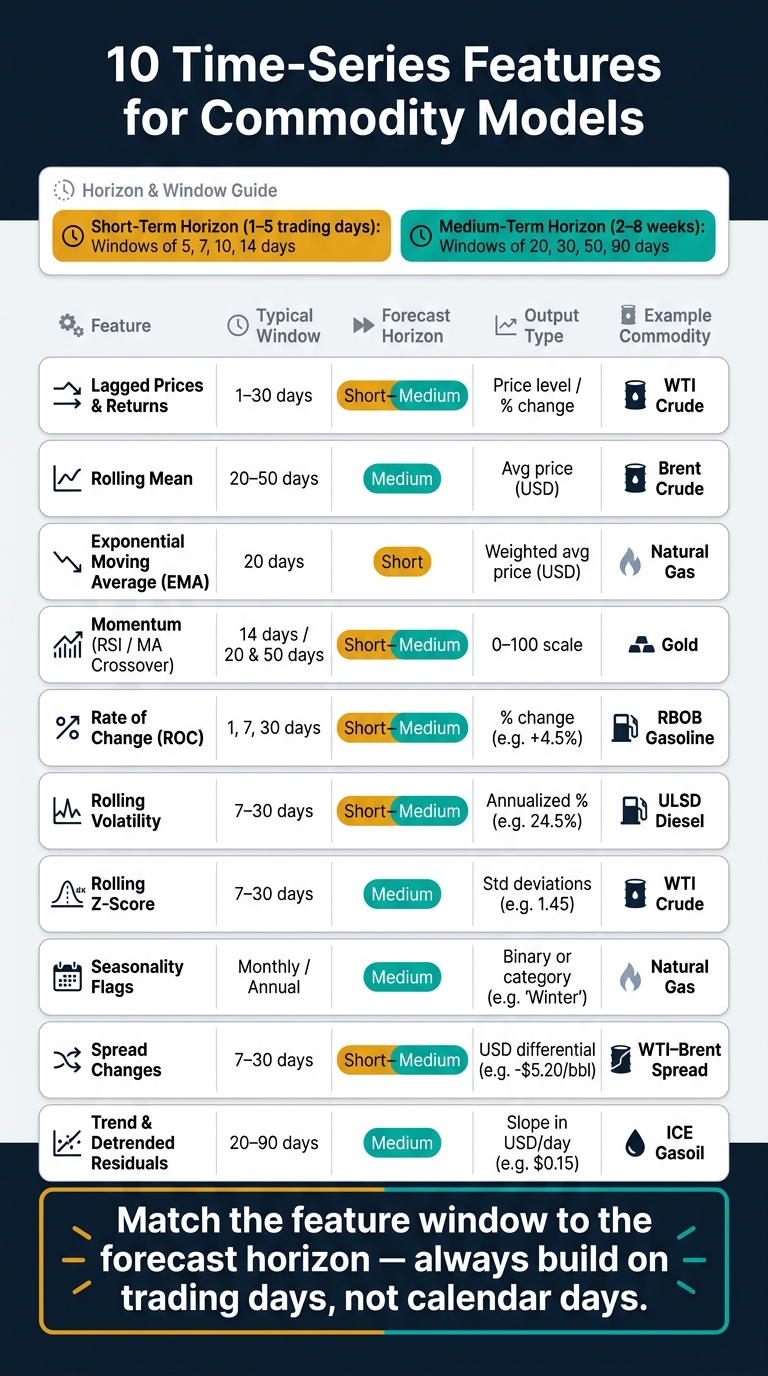
10 Time-Series Features for Commodity Models: Windows, Horizons & Use Cases
Quick Comparison
| Feature | Best Use | Common Window | Good For |
|---|---|---|---|
| Lagged prices/returns | Context and momentum | 1, 5, 7, 14, 30 days | Short to medium forecasts |
| Rolling mean | Smoothing trend | 20, 50 days | Medium forecasts |
| EMA | Faster trend signal | 20 days | Short forecasts |
| Momentum | Overbought/oversold and trend strength | 14, 20/50 days | Short to medium forecasts |
| ROC | Percent move speed | 1, 7, 30 days | Short to medium forecasts |
| Rolling volatility | Risk and market instability | 7, 30 days | Short to medium forecasts |
| Rolling z-score | Mean reversion and normalization | 7 to 14, 30 days | Short to medium forecasts |
| Seasonality flags | Recurring calendar effects | Monthly, yearly | Medium forecasts |
| Spread changes | Relative value | 7, 30 days | Short to medium forecasts |
| Trend/detrended residuals | Trend vs. deviation | 20, 30, 90 days | Medium forecasts |
A simple rule runs through the whole piece: match the feature window to the forecast window, and build on trading days, not calendar days. That keeps signals cleaner whether I’m working with WTI, natural gas, gold, or cross-market spreads.
sbb-itb-a92d0a3
What Makes a Good Commodity Time-Series Feature
A good feature tracks one repeatable market behavior. In commodities, that usually means momentum, trend, mean reversion, volatility, seasonality, or spreads.
The timing needs to fit the forecast window. For 1- to 5-day forecasts, use faster signals like 5-day or 10-day averages and short-term volatility. For 2- to 8-week forecasts, slower signals make more sense: 20-day to 50-day averages, 30-day volatility, and seasonality flags.
| Feature Type | Short-Term (1–5 Days) | Medium-Term (2–8 Weeks) |
|---|---|---|
| Moving Averages | 5-day or 10-day SMA/EMA | 20-day, 30-day, or 50-day SMA/EMA |
| Momentum | Z-Score | Seasonal patterns, trend strength |
| Volatility | Intraday price changes | 30-day rolling volatility |
| Sampling Interval | 1-hour or 1-day | 1-day or 1-week |
Your pipeline should follow trading days, not calendar days. That sounds small, but it matters. Commodity markets do not trade on a neat everyday schedule, so calendar-based handling can skew lags and rolling windows. Most benchmark contracts are priced in USD, which means spread features usually do not need currency conversion. And if you see a long-weekend gap, treat it as an exchange closure rather than missing data.
One more thing can trip people up: front-month rolls. They can create fake price jumps that look like market moves but aren't. To avoid that, tag each record by contract status before building lagged or rolling features. That keeps the first feature group clean: lagged prices and returns.
1. Lagged Prices and Returns
Lagged prices and lagged returns are two of the simplest inputs in commodity forecasting.
Lagged prices tell you where the market was. Lagged returns tell you how much it moved, in percentage terms.
Why It Helps
Commodity prices tend to drift over time. That makes raw price levels tougher for many models to handle on their own. Returns, by contrast, are usually more stationary, so they’re often easier to work with in forecasting models.
Signal Horizon
The time horizon matters more than the lag by itself.
For short-term momentum, lagged returns usually do the job better. For a broader read on trend direction, lagged prices give more context.
Window Length
The lookback window should line up with the forecast window.
- Use 7 to 14 days for short-term signals.
- Use 30 to 90 days for medium-term trend signals.
Commodity-Specific Use
Different commodities react at different speeds, and that changes how useful each lag can be.
Natural gas often needs shorter lags because weather shocks can hit fast. Gold often works better with longer lags that reflect a broader trend picture. In energy markets, aligned lagged series are also needed for crack-spread calculations.
These lagged inputs also feed the next feature group: rolling averages and EMAs.
| Lagged Prices | Lagged Returns | |
|---|---|---|
| Stationarity | Non-stationary | Generally stationary |
| Best Horizon | Medium to long-term | Short to medium-term |
| Primary Use | Trend context, turning points | Momentum, variance, correlation |
| Key Metric | SMA/EMA comparisons | Percentage change, log returns |
Once lagged values are set, smoothing them with rolling averages is the next step.
2. Rolling Mean
After lagged values, rolling means add smoothing. They help cut through day-to-day commodity price noise and make the main trend easier to spot.
Signal Horizon and Window Length
Use 5–10 days when you want fast signals that react to recent price moves. Use 20–50 days when you want a broader read on trend direction.
A common example is the 20-day average crossing above the 50-day average, which may point to upward momentum. The reverse may point to weakness. You can also use the smoothed series to build crossover, trend, and residual features downstream.
Stationarity Impact
Rolling means do not make prices stationary, but they can help remove trend when used as a baseline for residuals.
Commodity-Specific Use
Use SMA for steadier markets and EMA for faster-moving, trending markets. In energy markets, rolling means can help compare current spreads with recent history.
| Window Length | Sensitivity | Primary Use |
|---|---|---|
| Short (5–10 days) | High | Momentum signals, fast crossovers |
| Medium (20–30 days) | Moderate | Trend confirmation, volatility baselines |
| Long (50–200 days) | Low | Long-horizon trend tracking |
When you need a faster response to new prices, switch to EMA.
3. Exponential Moving Average (EMA)
EMA puts more weight on recent prices than SMA. So it reacts faster when a commodity starts to move. That makes it a good fit when direction right now matters more than long-run smoothing.
Signal Horizon
EMA tends to work best for short-term horizons of 1–7 days, where the latest price action often says more about the next move than older data does. For longer-horizon work, 20-day and 90-day windows are also common.
Window Length
A 20-day EMA is a solid choice for day-to-day trend tracking. If you're looking at slower, more seasonal energy series, stretching that window to 90 days usually makes more sense.
Commodity-Specific Use
EMA is often the better pick over SMA for fast-moving energy benchmarks like WTI and Brent. A simple way to use it is to track price against the EMA and watch for trend changes or stretched conditions. This gets even more useful when you pair it with a Z-score.
| Feature | SMA | EMA |
|---|---|---|
| Best For | Stable, low-volatility markets | Trending markets |
| Responsiveness | Slower; equal weight on all data | Faster; heavier weight on recent data |
| Primary Use | Long-term trend baseline | Short-term momentum and trend following |
EMA also helps shape momentum and rate-of-change features by giving those signals a smoother baseline.
4. Momentum
Building on EMA, momentum tells you if a move is picking up speed or running out of steam. That matters because a trend can still be in place while its energy starts to fade.
Signal Horizon
Momentum works across two time frames. For short-term reversal risk, use RSI. For medium-term trend confirmation, look at moving-average slope or crossover direction.
Window Length
The standard RSI setting is 14 days. For trend-following setups, a 20-day/50-day crossover is a common choice. A Golden Cross happens when the 20-day moves above the 50-day, which points to bullish trend strength. A Death Cross is the opposite and points to bearish trend strength.
| Indicator | Typical Window | Signal Horizon | Interpretation |
|---|---|---|---|
| RSI | 14 days | Short-term | >70 Overbought; <30 Oversold |
| MA Crossover | 20 & 50 days | Medium-term | Golden Cross (Bullish) or Death Cross (Bearish) |
Stationarity Impact
Bounded momentum indicators are often easier for models to learn than raw prices. Put simply, a tool like RSI stays within a fixed range, while price can drift all over the place.
Commodity-Specific Use
In oil, momentum can also help read spread pressure. In gas, though, you need to layer in seasonality. The same signal can mean one thing in one market and something else in another, so context matters when you read momentum across different commodity benchmarks.
Next, volatility shows whether that momentum is steady or unstable.
5. Rate of Change
Rate of Change (ROC) measures the percentage difference between the current price and the price a set number of periods ago. It sits somewhere between lagged returns and momentum because it shows how fast price moves are picking up.
Signal Horizon
ROC tends to work best for short- to medium-term trend shifts. That makes it handy when the speed of the move matters more than the move's direction by itself. Commodity models often use 1-, 7-, and 30-day horizons. A 7-day ROC can catch faster momentum shifts, while a 20- to 30-day window gives you more balance between responsiveness and stability.
Stationarity Impact
Because ROC expresses price movement as a percentage, it makes cross-commodity comparison much easier. Markets like WTI Crude and Natural Gas can be judged on the same percentage-change scale, which is the main reason ROC is useful in a multi-commodity model.
| Feature | Rate of Change (ROC) | Raw Price Data |
|---|---|---|
| Scale | High - comparable across commodities | Low - unit-dependent |
| Output | Percentage change | Price level |
Commodity-Specific Use
Use ROC on WTI, Brent, and natural gas to measure how fast prices are moving across markets.
Rolling volatility helps show whether those fast price changes are happening in a stable market or a shaky one.
6. Rolling Volatility
Once you know how fast price is moving, the next step is to measure how shaky that move is. That’s what rolling volatility does.
Rolling volatility measures the standard deviation of returns over a set window. If you're comparing daily series, annualize it with √252.
Signal Horizon
Rolling volatility works best for short- to medium-term risk signals, usually across 1-day to 30-day horizons. Forecasting systems often use it to build confidence intervals for 1-day, 7-day, and 30-day projections.
Window Length
For short-horizon signals, use a 7-day window. For most commodity models, 30 days is the default choice.
Commodity-Specific Use
This metric is especially helpful in energy markets and in mean-reversion models. In those settings, it helps with:
- VaR
- position sizing
- entry and exit timing
| Volatility Level | Annualized % | What It Means |
|---|---|---|
| Low | < 20% | Stable market |
| Moderate | 20%–40% | Normal fluctuation |
| High | > 40% | Unstable market |
When volatility gets high, mean-reversion signals tend to lose strength. That’s where the next feature, rolling z-score, starts to matter more.
7. Rolling Z-Score
When volatility makes raw prices tough to compare, a rolling z-score puts everything on the same scale. It shows how far the current commodity price is from its recent mean, measured in standard deviations. That makes it useful for mean reversion setups and spread signals.
Signal Horizon
The lookback window shapes the signal.
A 7- to 14-day window works best for short-term signals. It can catch fast price swings and near-term overbought or oversold conditions in high-volatility markets.
A 30-day window is a common default for medium-term analysis. It cuts down noise without giving up the short-term signal.
Commodity-Specific Use
Z-scores are especially helpful in spread analysis. For the WTI-Brent basis or the 3-2-1 crack spread, a z-score far from zero suggests the spread is unusually wide or tight. That can point to a mean reversion trade or an arbitrage setup.
| Z-Score Range | Market Condition | Model Interpretation |
|---|---|---|
| > 2.0 | Extremely overbought | Potential overbought signal |
| 1.0 to 2.0 | Above average | Monitor for reversal |
| -1.0 to 1.0 | Normal range | Neutral / hold |
| -2.0 to -1.0 | Below average | Monitor for entry |
| < -2.0 | Extremely oversold | Potential oversold signal |
The same normalization can also help spot seasonal shifts and changes in spreads.
8. Seasonality Flags
After z-score normalization, add calendar flags to pick up recurring demand cycles. These flags are simple binary or category markers that show where a date sits on the calendar. In plain English, they tell the model things like month, day, and rollover timing (similar to how ChatGPT analyzes oil prices) so it can use those patterns directly.
Signal Horizon
Seasonality flags tend to help most with medium-term predictions, especially around the 30-day horizon. That makes sense: over 30 days, recurring demand cycles have enough time to show up in prices.
Commodity-Specific Use
Natural Gas is the clearest case where seasonality flags matter. Prices often move in monthly patterns tied to winter heating demand and summer cooling demand. If you're modeling natural gas, pull the month from the timestamp and average monthly prices across at least 3 years to spot recurring seasonal peaks.
Refined products such as heating oil often show a similar winter demand pattern. And for futures-based models, add a rollover flag so you keep the contract context instead of blending one contract period into another.
Pair seasonality with z-scores to test whether a seasonal move is normal or stretched. A z-score above 2.0 indicates the price is significantly overvalued relative to its 30-day mean.
This setup also works well with spread changes, since spreads help show relative value between benchmarks.
| Commodity | Main Driver | Key Flags |
|---|---|---|
| Natural Gas | Weather (Heating/Cooling) | Month-of-year, weather seasons |
| Refined Products | Seasonal Consumption | Winter demand seasons |
9. Spread Changes
Once you’ve added seasonality flags, spread changes help the model move beyond one price at a time. Now you’re looking at relative value between related contracts.
A spread is the gap between two related prices and the way that gap changes over time. In commodities, that gap can say more than either price on its own. That’s why spreads matter so much. They give the model steadier inputs, make cross-market comparisons easier, and help flag odd moves when you're trying to predict direction, mean reversion, or relative value.
Signal Horizon
Spreads work well for short-term anomaly detection and arbitrage setups. They also fit medium-term use cases, like crack spreads and basis differentials tied to planning and risk management.
Window Length
For fast spread moves, use a 7-day window. For baselines like the mean, standard deviation, and z-score, a 30-day window is a solid starting point. Longer lookbacks make sense for calendar spreads and energy ratios, where moves can play out over more time.
Stationarity Impact
Spreads are often more stationary than raw prices. That makes them a good fit for mean-reversion and relative-value models. In plain English: they’re often easier to model when you care about entry and exit points based on relative mispricing.
Commodity-Specific Use
Not every commodity spread works the same way. Some are better for arbitrage, others for refinery economics or curve structure. Here are the pairings that tend to be the most useful:
| Spread Type | Example | Best Use |
|---|---|---|
| Basis Spread | WTI minus Brent | Arbitrage and regional pricing |
| Crack Spread | 3-2-1 (2 × gasoline + 1 × heating oil − 3 × crude) | Refining margin analysis |
| Calendar Spread | ICE Brent nearby vs. deferred month | Contango/backwardation monitoring |
| Energy Ratio | Gas-to-oil thermal equivalent ratio | Fuel switching and macro research |
If a spread still shows a trend even after normalization, that usually means the trend itself deserves to be modeled directly.
10. Trend and Detrended Residuals
Trend and detrended residuals break a price series into two parts: direction and deviation. The trend shows where price has been heading. The residual shows what remains once that trend is stripped out.
This is useful when raw prices look messy and hard to read. Instead of staring at every wiggle, you get a cleaner split between trend-following behavior and mean reversion.
Stationarity Impact
Raw prices are non-stationary, which makes them harder to work with in many models. Detrending removes directional bias, so reversals stand out more clearly.
Signal Horizon
Detrended residuals tend to work best for medium-term mean-reversion setups, usually around a 30-day horizon. That window often gives enough time for deviations from trend to show up without getting buried in day-to-day noise.
For broader shifts in market direction, longer windows in the 30-day to 90-day range give a steadier read on slope and strength. A 7-day horizon can still pick up faster reversal moves, but it tends to be noisier.
Window Length
A 20-day window is a good default for smoothing trend calculations.
Commodity-Specific Use
In commodities, detrended residuals help split trend from reversion in:
- WTI
- Brent
- natural gas
- refined-product spreads
The table below compares detrended residuals with the other nine feature types by signal type and horizon.
Feature Comparison Table
The table below sums up all 10 features by window, horizon, and output scale. Use it to pick the shortest window that still fits your forecast horizon.
| Feature | What It Measures | Typical Window | Horizon | Example Output | Example Commodity |
|---|---|---|---|---|---|
| Lagged Prices and Returns | Prior price/return | 1- or 5-day window | Short | $78.45 (USD) | WTI Crude Oil |
| Rolling Mean | Average price | 20, 50 trading days | Medium | $72.45 (USD) | Brent Crude |
| Exponential Moving Average | Price-weighted average | 20 trading days | Short | $73.12 (USD) | Natural Gas |
| Momentum | Speed of price change | 14 trading days | Short | 62.5 (0–100 scale) | Gold |
| Rate of Change | Percent change | 1 day, 30 days | Short | +4.5% (Percent change) | RBOB Gasoline |
| Rolling Volatility | Price fluctuation | 30 trading days | Medium | 24.5% (Annualized %) | ULSD Diesel |
| Rolling Z-Score | Std. deviations from mean | 30 trading days | Medium | 1.45 (Standard deviations) | WTI Crude Oil |
| Seasonality Flags | Calendar-based patterns | Monthly or annual | Medium | 1 (Binary) or "Winter" | Natural Gas |
| Spread Changes | Price differential | Daily | Short | -$5.20 (WTI-Brent USD/bbl) | WTI-Brent Spread |
| Trend and Detrended Residuals | Slope & strength | 30, 90 trading days | Medium | $0.15 (Slope in USD/day) | ICE Gasoil |
This makes the main idea pretty simple: short-horizon forecasts usually lean on shorter windows, while medium-horizon forecasts often need a bit more history. If you're deciding between two setups, start with the shorter window that still lines up with the forecast period you're targeting.
Next, apply these feature windows to live benchmark data.
How to Apply These Features to Real Commodity Data
Use the feature windows above as a simple template for building clean commodity inputs.
Before you calculate any feature, get the data lined up and cleaned. Holiday gaps and exchange closures can throw off rolling features in a big way. If timestamps don’t match, your lags, rolling means, volatility, z-scores, and spreads can end up reflecting calendar noise instead of market movement. That’s why it helps to align feeds first, especially around U.S. market holidays and exchange closures.
For the features themselves, use each input for the job it handles best:
- Returns for scale-free risk and volatility inputs
- Prices for moving averages and trend signals
- Z-scores to compare commodities on the same scale
Window length should match the forecast horizon. If you’re working with daily data, annualize daily volatility with √252. And this part matters: use only the data available at each timestamp. No peeking ahead. When scaling inputs, fit scalers on the training set and then apply those same scalers to the test set.
A benchmark feed also makes this much easier to run in both live and historical pipelines. OilpriceAPI provides real-time and historical benchmark data for Brent, WTI, Natural Gas, and Gold in JSON.
Conclusion
No single feature works in every market state. Markets move between stable, trending, and uncertain periods, and a signal that looks strong in one setting can fall apart in another.
Feature choice also depends on forecast horizon. Short-term models lean more on lags, momentum, and near-term volatility. Medium-term models get more from longer rolling averages, seasonal flags, and spread signals that tend to stick around.
Using a mix of methods helps cut the risk of overfitting to one market state. That mix gives commodity models a better shot at holding up as conditions change.
FAQs
Which features should I start with for a 1- to 5-day commodity forecast?
For a 1- to 5-day commodity forecast, start with features that reflect near-term momentum and volatility. Focus on:
- Momentum indicators like RSI and SMA/EMA
- Volatility metrics for short-term swings
- Current spread data, such as basis or crack spreads
These features help track immediate trend direction, market intensity, and relative price moves.
How do front-month rolls and holiday gaps affect time-series features?
Front-month rolls and holiday gaps can create artificial breaks in time-series data that throw off technical indicators. A contract roll can look like a sudden momentum change or a volatility jump. Holiday gaps can also warp rolling means and z-scores that assume the data is continuous.
To keep forecasting models accurate, analysts need data pipelines that handle these breaks and preserve contract-month context.
When should I use z-scores or spread changes instead of raw prices?
Use z-scores for spread changes instead of raw prices when you want to tell whether a current price gap is statistically meaningful compared with its past average.
Raw prices show the nominal spread. Z-scores normalize that spread by showing how many standard deviations it sits above or below the historical mean. That makes it much easier to spot possible overbought or oversold conditions, along with setups that may be due for a reversal.