If you want to judge a gas CCS project fast, follow one rule: track the CO2 from source to storage. A case study only means much if it covers the whole chain: source, transport, and geologic storage.
I’d read any gas CCS buildout through five simple checks:
- Map the chain: where CO2 comes from, how it moves, and where it is injected
- Check the source type: gas processing, NGCC, SMR, or LNG all have different cost and design limits
- Track the timeline: FEED, FID, first injection, and post-injection monitoring
- Split the cost stack: capture, transport, and storage in $/tCO2
- Use shared KPIs: capture rate, injected tons, uptime, injectivity, and cost per ton avoided
A few numbers frame the topic. As of September 2023, the U.S. had 15 CCS facilities with about 22 million metric tons per year of capacity, or about 0.4% of U.S. emissions. For gas-fired power plants, flue gas is only about 3%–4% CO2, which makes separation harder than at gas processing units. And in the U.S., a Class VI storage permit can take around 24 months, so storage often sets the schedule.
Here’s the short version of what matters most:
- Project boundary comes first. A capture-only project view can hide transport or storage limits.
- Volumes must match. Gross emissions, captured CO2, and stored CO2 are different numbers.
- Transport can swing costs. Distance, terrain, offshore routing, and pipe reuse all matter.
- Storage fit is non-negotiable. Injectivity has to match planned CO2 supply.
- Gas price matters. As of August 6, 2026, Henry Hub is $2.75/MMBtu, with a 12-month average of $3.34/MMBtu and a 12-month range of $2.68 to $4.46/MMBtu.
Carbon capture breakthrough: 99% at $20/MWh premium | Interchange Recharged
sbb-itb-a92d0a3
Quick Comparison
| What to check | What I’d look for | Why it matters |
|---|---|---|
| Source | NGCC, gas processing, SMR, LNG | Source type shapes CO2 purity, energy use, and cost |
| Transport | Feeder line, trunk line, repurposed pipe, ship | Route and distance affect cost and timing |
| Storage | Saline formation, depleted field, EOR | Storage type affects injectivity, permits, and monitoring |
| Timeline | FEED, FID, first injection | Shows project maturity and delay risk |
| Economics | Capture, transport, storage in $/tCO2 | Makes side-by-side comparison cleaner |
| KPIs | Capture rate, uptime, injected tons, pressure data | Helps track actual project performance |
Put simply, I’d use this guide as a screening tool: Does the project connect a real source to a real sink, on a real schedule, with numbers that line up? If yes, the case study is worth a closer look.
Map the Chain: Sources, Transport Corridors, and Storage Sinks
Once the project boundary is set, the next step is mapping the full source-to-sink chain.
A good asset map lets you size up the project fast. Before you get into cost numbers or schedule details, look for three basics:
- where CO₂ is captured
- how it moves
- where it ends up
That layout tells you a lot right away. You can usually tell whether you're looking at a single-site retrofit, a shared hub for several emitters, or a greenfield project where capture, transport, and storage are all being built from the ground up.
Identify capture assets and annual CO₂ volumes
Not all CO₂ sources work the same way, and that shapes how you read the map.
Gas processing units remove CO₂ from feed gas through acid gas removal. That usually creates a high-purity CO₂ stream, so the main capture work often centers on dehydration and compression. NGCC power plants are a different story. They emit dilute flue gas, with CO₂ concentrations of about 3%–4% by volume, which means large amine systems and a lot of energy for solvent regeneration. In plain terms, gas processing units tend to produce high-purity CO₂ streams at lower capture cost, while NGCC flue gas is dilute and costs more to capture.
Hydrogen and steam methane reforming (SMR) units add another layer. They produce two CO₂ streams: a high-concentration process gas that is above 95% CO₂, plus a more dilute flue gas from burners. If a project captures only the process gas, it leaves out a big share of total emissions. So when you read a case study, check whether it says exactly which streams are included.
On the map, look for the annual CO₂ volume per source, usually shown in MtCO₂/year. Then check what that number means. It may refer to:
- gross emissions
- captured CO₂
- net stored CO₂
Those are not the same figure, and mixing them up can throw off the whole read.
After that, follow the transport corridor.
Trace CO2 pipelines, repurposed gas lines, and marine routes
Most case study maps separate CO₂ trunk lines, feeder lines, and repurposed gas infrastructure through line style, labels, or the legend.
Trunk lines usually serve several sources. They tend to appear as thick central lines with branch connections and higher capacity. Feeder lines are smaller links from one plant to a trunk line or straight to storage. Repurposed gas lines may be labeled as converted natural gas pipelines. When you trace these routes, pay attention to corridor length, diameter, design pressure, and throughput. Also watch for notes on integrity upgrades, pressure changes, or diameter limits.
Transport cost is driven by distance and terrain more than many people expect. Onshore CO₂ pipelines over 250 km can cost from $1.30 to $10.90 per metric ton, while offshore pipelines over similar distances run from $1.90 to $14.80 per metric ton.
Marine routes come into play when storage is offshore. In those cases, the map should show loading terminals, ship capacity, and voyage timing. Vessel sizes are typically 30,000–40,000 m³ per vessel, and round-trip time matters because it affects fleet size and the cost per ton. The U.S. Department of Energy has noted that a large-scale steel pipeline network is likely the most practical and cost-effective route to gigaton-scale CCS, given the limits of truck, rail, and shipping at high volumes.
Locate storage sites and check source-to-sink fit
Storage sites usually appear as fields or geologic formations, such as saline aquifers, depleted gas reservoirs, or EOR sites. Maps often label them with permitted capacity in MtCO₂, injectivity in MtCO₂/year, and project status.
The key check here is simple: does the storage site's injectivity match or exceed the total captured CO₂ being sent to it? If captured volumes are higher than injectivity, the case study should spell out how that gap is handled. It also helps to confirm the storage status - whether it is at the application stage, permitted, or already operating.
The table below sums up how source type, transport mode, and storage type come together across different project setups. It's a handy side-by-side reference when you're comparing case studies.
| Project Type | Capture Source | Transport Mode | Storage Type | Integration Notes |
|---|---|---|---|---|
| Single-site retrofit | NGCC power plant | New feeder pipeline | Depleted gas field | Capture added to an existing plant; dedicated storage link |
| Gas processing hub | Natural gas processing unit | Trunk CO₂ pipeline | Deep saline aquifer | High-purity stream; multiple processing trains connected |
| SMR hydrogen facility | Steam methane reformer | Repurposed gas line | EOR reservoir | Process gas captured; flue gas may be excluded |
| LNG terminal (multi-stream) | LNG feed gas and combustion emissions | Pipeline + marine route | Offshore saline formation | Mixed-stream complexity; marine leg to offshore sink |
| Greenfield cluster | NGCC + gas processing | New trunk + feeder lines | Saline aquifer | All assets under development; future expansion capacity |
Once the chain is mapped, the next check is which assets are already permitted, built, or still in FEED.
Follow the Project Lifecycle from FEED to Injection
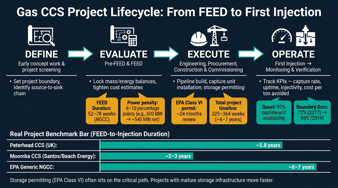
Gas CCS Project Lifecycle: From FEED to First Injection
A gas CCS case study makes more sense when you read it as a chain of stages: define, evaluate, execute, and operate. That framing helps you judge two things fast: how mature the project is and where schedule risk is likely to sit. After that, the key job is simple: map the milestones and see how far the project has actually moved.
The define stage covers early concept work and project screening. The evaluate stage includes pre-FEED and FEED, where engineering teams lock down mass and energy balances, tighten cost estimates, and sort out how the CCS system fits with existing gas assets. Execute covers detailed engineering, procurement, construction, and commissioning. Operate starts at first injection and continues through routine monitoring and verification.
Capture design and plant integration
In FEED, the case study should spell out the solvent system, put numbers on the power penalty, and show how heat integration supports regeneration. It should also deal with practical site limits, like tight plot space at LNG facilities or amine-unit upgrades at gas-processing plants.
For NGCC plants, the power penalty is one of the clearest signals to watch. A drop of about 6–10 percentage points in net efficiency is normal. In plain terms, that can mean going from 600 MW to about 540 MW net. Heat integration diagrams matter too. They show whether low-grade steam or waste heat from gas turbines or compression trains is being used for solvent regeneration. That detail has a big effect on efficiency and on whether a retrofit is even workable. If a case study glides past those points, that's a reason to be careful.
Once the capture setup is pinned down, the schedule often shifts to transport and storage.
Transport development and storage permitting
Transport and storage permitting often sit on the critical path. For pipelines, check whether the project relies on a new dedicated CO2 line or a repurposed natural gas pipeline. Then look for the nuts-and-bolts details: diameter, length in miles, design pressure in psig, and material specs. If an old gas line is being reused, the case study should mention integrity checks for fracture control and CO2 corrosion compatibility. If it doesn't, that's a gap worth marking.
In the U.S., dedicated storage projects need EPA Class VI permits, and review can take about 24 months.
Timeline milestones that matter
When you compare projects, four dates tend to tell the story:
- FEED completion
- FID
- first injection
- any stated closure date or post-injection monitoring start
The most useful schedule check is the gap between FEED completion and first injection. EPA schedule data for NGCC projects puts FEED at 52–78 weeks, while full project timelines run 325–364 weeks, or about 6–7 years. So if a project claims a much shorter path, it should clearly explain how it handles storage permits, right-of-way approvals, and retrofit complexity. Otherwise, the numbers may be doing a bit too much heavy lifting.
The table below shows how those milestones line up across similar projects, with FEED-to-injection duration as a quick comparison measure.
| Project | FEED Completion | FID | First Injection | FEED-to-Injection |
|---|---|---|---|---|
| Peterhead CCS (UK) | Feb 24, 2014 | Targeted Dec 14, 2015 | Dec 4, 2019 | ~5.8 years |
| Moomba CCS (Santos/Beach Energy) | FID reached on $165 million project | Confirmed | Targeted 2024 | ~2–3 years (mature gas-field storage) |
| EPA Generic NGCC Schedule | FEED 52–78 weeks | Included in gate model | Startup, commissioning, and testing phase | 325–364 weeks total (~6–7 years) |
Peterhead is a good reference point. Even though its FEED agreement took effect in February 2014, first injection did not happen until December 2019. That's almost six years. Moomba CCS, backed by Santos and Beach Energy, reached FID on a $165 million project and reported full lifecycle costs below $24 per metric ton of CO2, in part because existing gas-field infrastructure cut down the greenfield scope. That pattern shows up again and again: projects with mature storage infrastructure or co-located sinks tend to move from FEED to injection faster than greenfield builds.
With schedule risk mapped, the next comparison is cost.
Read the Economics: Cost Drivers, Price Signals, and Sensitivities
Once the project path is clear, the next step is simple: check whether the numbers still make sense at scale. That’s where project economics earns its keep. It helps you tell the difference between a gas CCS buildout that looks workable and one that sounds fine in a slide deck but falls apart in practice.
Break total cost into capture, transport, and storage
Start by splitting project economics into three buckets: capture, transport, and storage. In most cases, capture is the biggest cost item. Transport and storage are often more sensitive to pipeline distance, project scale, throughput, and reservoir conditions.
Use $/tCO2 for capture and storage, $/kW for plant capital, and $/MMBtu for fuel. Then convert energy prices to $/MWh when you compare projects across countries. That avoids unit mix-ups and makes side-by-side analysis much cleaner.
| Unit | Context | Application |
|---|---|---|
| $/tCO2 | Carbon markets, project finance | Avoided cost, capture cost, storage fees |
| $/kW | Power generation | Capture plant integration |
| $/MMBtu | U.S. natural gas markets | Fuel input cost, operating expense modeling |
| $/MWh | Global comparison | Normalized unit for cross-border analysis |
Once those buckets are in place, normalize the inputs before you run gas-price scenarios. If you skip that step, comparisons can get messy fast.
Use natural gas price data in scenario analysis
Natural gas price is one of the biggest variables in gas CCS sensitivity modeling. When gas prices move, plant run time can change. And when run time changes, captured volume changes too. At a gas-fired power plant, Henry Hub prices shape dispatch economics, which then affects how often the CCS system is online.
As of August 6, 2026, Henry Hub natural gas is priced at $2.75/MMBtu, down 8.94% year over year. The 12-month average is $3.34/MMBtu, and the 12-month range runs from $2.68 to $4.46/MMBtu. That kind of swing can change CCS margins in a big way. A yearly average may look calm, but it can hide the risk that shows up during price spikes.
If you want to test this with actual market data, OilpriceAPI provides JSON REST access to real-time and historical natural gas prices through the NATURAL_GAS_USD commodity code. You can use GET /v1/prices/past_year with 1d or 1w intervals to backtest CCS utilization against Henry Hub volatility using commodity price data in LLMs.
Compare costs across projects with a standard table
Project comparisons only hold up when each case uses the same unit system. The cleanest approach is to normalize capture, transport, and storage to $/tCO2 and then flag the main sensitivity in each bucket.
| Cost bucket | Preferred unit | Main sensitivities |
|---|---|---|
| Capture | $/tCO2 | Capture rate, plant size |
| Transport | $/tCO2 | Pipeline distance, throughput |
| Storage | $/tCO2 | Reservoir characteristics, storage geology |
This kind of table makes it much easier to spot what’s driving the gap between projects. In one case, the issue may be capture cost. In another, transport distance or storage geology may be doing the damage. Those normalized costs then become the starting point for the operating KPIs that follow.
Track Operating Metrics and API-Ready Data Points
Once costs are normalized, move from project economics to measured performance. The goal is simple: use the same core KPIs across capture, transport, and storage so each case study can be compared on equal terms.
Core KPIs for performance and verification
Track capture rate, CO2 captured, transported CO2, injected CO2, uptime, injectivity, storage utilization, and cost per ton avoided. That last metric matters more than cost per ton captured because it also reflects compression and capture energy.
Project data helps ground this. Quest reported 97% capture-unit availability and over 99% compressor-unit availability during its first two full years. Boundary Dam moved from 72% of planned capture in 2017 to 95% in 2019. That’s why multi-year trendlines matter more than a one-year snapshot.
It also helps to track captured, transported, and stored CO2 as separate figures. When those numbers don’t line up, the gap usually points to venting, downtime, pipeline limits, or injection stoppages.
Monitoring, reporting, and data schema design
After throughput, the next step is MRV. For subsurface reporting, track reservoir pressure, wellhead pressure, annulus pressure, plume extent, and well integrity tests. U.S. EPA guidance for Class VI geologic sequestration wells calls for continuous recording of injection pressure, injection rate, injection volume or mass, temperature, annulus pressure, and annulus fluid volume. California's CCS protocol says continuous means at least one measurement every 15 minutes for some parameters.
If you're building a data warehouse or dashboard, the minimum schema should include both raw measurements and calculated fields. Raw fields should cover timestamps, units, sensor type, reporting period, and project phase. Calculated fields can include capture efficiency, storage efficiency, and cumulative totals.
One field you should NEVER skip: verification status. Add source document type too. That makes it much easier to tell operator-reported numbers from regulator filings or third-party-verified figures.
Use the same fields in every case study. It keeps comparisons clean and makes dashboards far easier to query.
| KPI Name | Definition | Unit | Reporting Frequency | Primary Data Source |
|---|---|---|---|---|
| Capture rate | % of inlet CO2 removed at the capture unit | % | Monthly | Plant instrumentation, MRV plans |
| Mass captured | Total CO2 isolated from the gas stream | Metric tons (tCO2) | Monthly | Flow meters, MRV filings |
| Mass injected/stored | CO2 successfully delivered to the storage formation | Metric tons (tCO2) | Monthly/Quarterly | Regulator filings, monitoring reports |
| Uptime/availability | % of time the capture asset was operational | % | Monthly | Technical performance summaries |
| Injectivity | Rate at which the reservoir accepts CO2 | tCO2/day | Monthly | Monitoring and modeling reports |
| Annulus pressure | Pressure in the well annulus as an integrity indicator | psi | Continuous | Well monitoring, MIT records |
| Storage utilization | Cumulative injected CO2 ÷ permitted storage capacity | % | Quarterly | Operator or regulator filings |
| Cost per ton avoided | Total project cost divided by net CO2 avoided | $/tCO2 | Annual | Project economics reports |
If project economics shift with gas prices, connect the price series through OilpriceAPI so margin swings have a clear explanation.
Conclusion: A checklist for comparing gas CCS case studies
Before closing out a case study, run five checks:
- Map the full chain: source asset, capture unit, transport corridor, injection site, and storage formation.
- Read maps from source to sink and make sure CO2 volumes, pipeline routes, and storage geology are all accounted for.
- Align milestones to lifecycle stages: FEED, FID, first injection, and steady-state operation each come with different data quality and comparison limits.
- Separate cost buckets into capture, transport, and storage using $/tCO2 as the common unit.
- Extract standardized metrics with clear units, reporting cadence, and source type for dashboard or API use.
The case studies that stand up to scrutiny usually share the same traits: captured, transported, and stored volumes are reported separately, multi-year trends are visible, and the schema is clean enough to query.
FAQs
Why isn’t capture rate enough?
Capture rate on its own doesn't tell you enough about natural gas CCS buildouts. To judge whether a project can work, you also need to look at asset connectivity, regional transport links, and cost signals.
That bigger picture matters. If you only focus on technical capture specs, you can miss whether the project actually makes economic sense.
So it helps to track the broader commodity price environment alongside infrastructure data. That gives you a much better read on whether a CCS project is viable in practice, not just on paper.
What makes storage the main bottleneck?
Storage is one of the biggest choke points for natural gas. Unlike oil, stranded gas doesn't have many local storage options. So when output rises above pipeline takeaway capacity - especially with associated gas from oil drilling - producers can hit a wall fast.
That pressure creates a harsh trade-off. If companies don't want to shut in profitable oil production, they may end up paying others to take the gas off their hands. And when that happens, hub prices can sink deep into negative territory.
How do gas prices affect CCS economics?
Natural gas prices have a direct impact on whether carbon capture and storage (CCS) projects make business sense. They shape day-to-day operating costs and affect how competitive CCS-equipped facilities are against other options in the market.
When gas prices are low - or even negative - the push to invest in efficiency upgrades or capture systems can weaken. On the flip side, when prices climb, the energy-heavy nature of carbon capture can get a lot more expensive.
OilpriceAPI can help track these shifts, which makes it easier to assess project feasibility over time.